1.2 Modèle utilisé

Le modèle en tangage-pilonnement

Le schéma de principe Zoom$\downarrow $

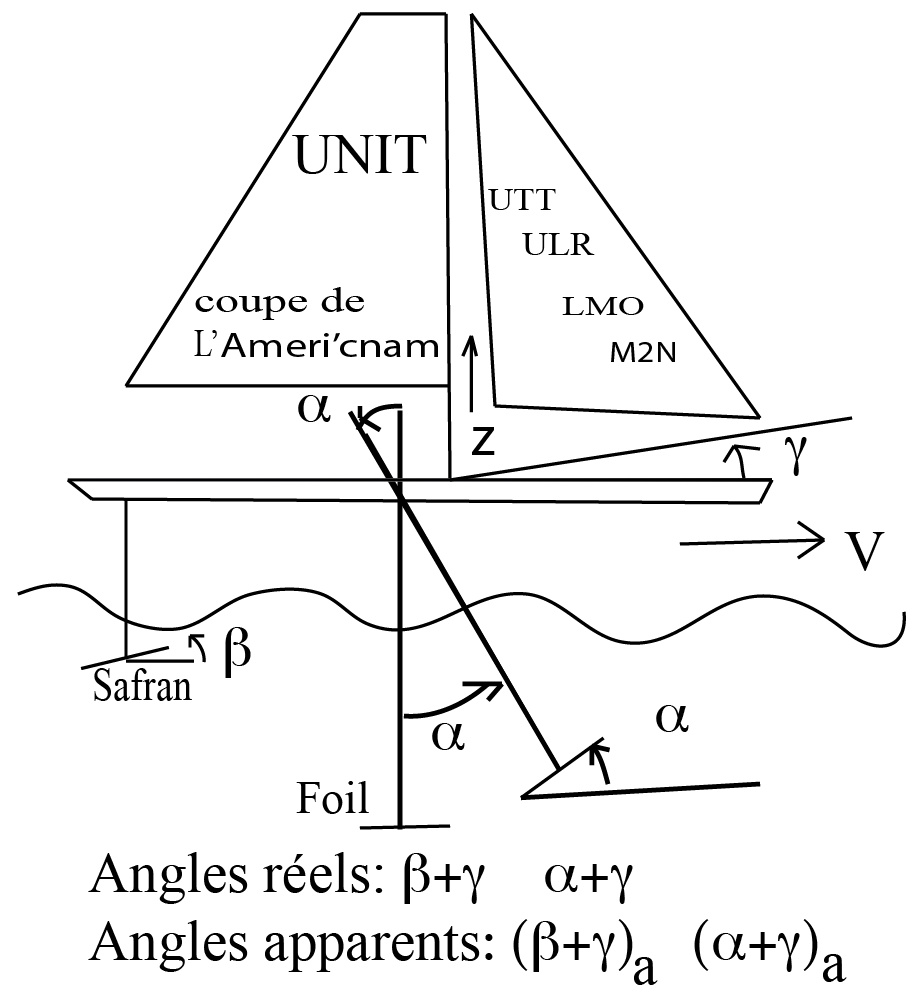
Le schéma de montage in situ

2DDL: le tangage est $\gamma $, le pilonnement en $O$ est $z$; $\beta $ fixé, $\alpha $ le contrôle
($G$ est en arrière du pont $O$ si $a{>}0$ et en avant si $a{<}0$; les moments sont estimés en $O$.)

\[ \hskip-11.9501574803pt\boxed { \begin{array}{l} M\ddot z\hskip-2.84527559055pt-\hskip-2.84527559055ptaM\cos (\gamma )\ddot\gamma \hskip-2.84527559055pt=\hskip-1.42263779528pt-Mg\hskip-2.84527559055pt+\hskip-2.84527559055pt\frac{\varrho S_ s \vert V_{as}\vert ^2}{2}c_{zs}((\beta \hskip-2.84527559055pt+\hskip-2.84527559055pt\gamma )_ a)\hskip-2.84527559055pt+\hskip-2.84527559055pt\frac{\varrho S_ f \vert V_{af}\vert ^2}{2}c_{zf}((\alpha +\gamma )_ a),\\ -aM\cos (\gamma )\ddot z \hskip-2.84527559055pt+\hskip-2.84527559055ptJ_0\ddot\gamma \hskip-2.84527559055pt=\hskip-1.42263779528pt-M_0\hskip-1.42263779528pt+\hskip-2.84527559055pt\frac{\varrho S_ sL \vert V_{as}\vert ^2}{2}c_{ms}((\beta \hskip-2.84527559055pt+\hskip-2.84527559055pt\gamma )_ a)\hskip-2.84527559055pt+\hskip-2.84527559055pt\frac{\varrho S_ fL \vert V_{af}\vert ^2}{2}c_{mf}((\alpha \hskip-2.84527559055pt+\hskip-2.84527559055pt\gamma )_ a)\\ \hskip-8.53582677165pt~ ~ +\hskip-2.84527559055pt\frac{\varrho }{2}\big [S_ fd_ f\sin (\alpha \hskip-2.84527559055pt+\hskip-2.84527559055pt\gamma )\vert \hskip-0.56905511811ptV_{af}\hskip-0.56905511811pt\vert ^2c_{zf}((\alpha \hskip-2.84527559055pt+\hskip-2.84527559055pt\gamma )_{a})\hskip-2.84527559055pt-\hskip-2.84527559055ptS_ s(h\cos (\gamma )\hskip-2.84527559055pt-\hskip-2.84527559055ptd_ s\sin (\gamma ))\vert \hskip-0.56905511811ptV_{as}\hskip-0.56905511811pt\vert ^2c_{zs}((\beta \hskip-2.84527559055pt+\hskip-2.84527559055pt\gamma )_{a})\big ]\end{array}} \]